Hands-on linear regression for machine learning
Goal
This is the sharing session for my team, the goal is to quick ramp up the essential knowledges for linear regression case to experience how machine learning works during 1 hour. This sharing will recap basic important concepts, introduce runtime environments, and go through the codes on Notebooks of Azure Machine Learning Studio platform.
Recap of basic concepts
Do not worry about these theories if you can’t catch up, just take it as an intro.
Steps of machine learning
- Get familiar with dataset, do preprocessing works.
- Define the model, like linear model or neural network.
- Define the goodness/cost of model, metrics can be error, cross entropy, etc.
- Calculate the best function by optimization algorithms.
Linear model
Let’s start with the simplest linear model
Question: How to initialize parameters?
Generalization
The model’s ability to adapt properly to new, previously unseen data, drawn from the same distribution as the one used to create the model.
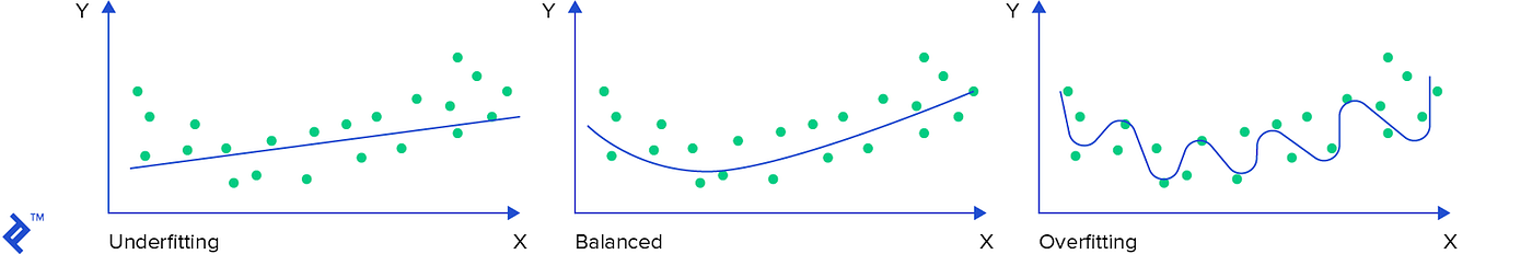
- Underfitting: model is too simple to learn the underlying structure of the data (large bias)
- Overfitting: model is too complex relative to the amount and noisiness of the training data (large variance)
Solutions: References and resources, or Underfitting and Overfitting in machine learning and how to deal with it.
Loss/Cost function
There is a dataset for training, it looks like:
Obviously the smaller loss, the better model. So our target function should be:
Average value would be better than total sum, then we get the actual function that needs to be computed:
Not big deal, just minimize the mean square error of our trivial linear model.
Vectorized form
You may have heard “feature” before, for each of data
Kind of verbose right? Let’s use
Thus our loss function of vectorized form is:
Notice that
In addition, deep learning depends on matrix calculations especially, it will take advantage of GPU to speed up model training.
Closed-form solution
As we already know the values of
Check out this online course video (about 16min) from Andrew Ng to learn more.
Yes we’re done. Our introduction is here 🤣🤣🤣 .
Question: How to deal with complex models? How about computation burden?
Gradient Descent
Gradient Descent is a generic optimization algorithm capable of finding optimal solution to a wide range of problems.
Gradient descent is a first-order iterative optimization algorithm for finding a local minimum of a differentiable function.
Our loss function is differentiable indeed, so we can use it to find the local minimum (also the global minimum in this case). Let’s get it by one chart.
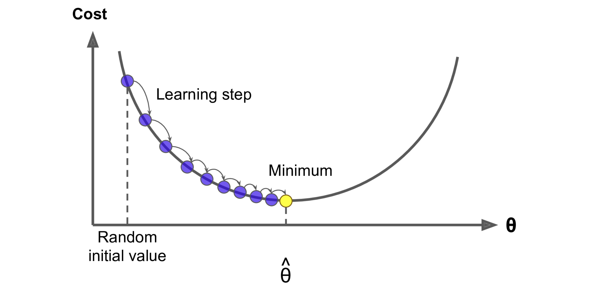
So here is the last equation in this post (I promise, typing these LaTeX expressions really wore me out 🥲 ), the gradient of our loss function:
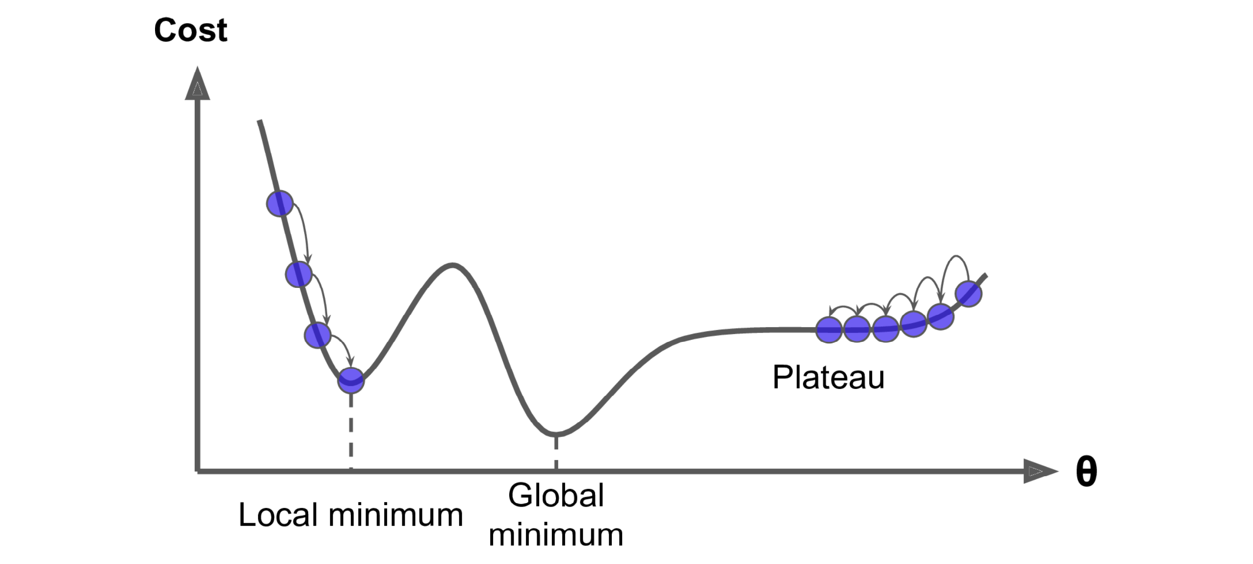
Question: disadvantages of gradient descent?
Variants optimizers
- SGD, Stochastic gradient descent
- Adam
- Mini-batch gradient descent
- Adagrad
Training tips
Probably it’s enough for us to dig into the code, so the recap should be stopped here. At last, giving this tips section for some practical training techniques.
- Hyperparameters tuning/optimization, like pick a good learning rate
- L2 (Ridge) regularization
- Early stopping
- Feature engineering
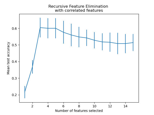
- Feature selection by recursive feature elimination and cross-validation (RFECV)
![Recursive feature elimination with cross-validation, https://scikit-learn.org]()
- Feature scaling like normalization
- Data correction for dirty part
- Defining and removing outliers
- Update model to make it fits dataset better like add high order term for most important feature, or even you can use a neural network if you want 😏
- Feature selection by recursive feature elimination and cross-validation (RFECV)
- Leveraging K-fold cross validation to split data and evaluate model performance
Runtime environments
Local
I highly recommend using Conda to run your Python code even on Unix-like OS, and Miniconda is good to get start.
Conda as a package manager helps you find and install packages. If you need a package that requires a different version of Python, you do not need to switch to a different environment manager, because conda is also an environment manager. With just a few commands, you can set up a totally separate environment to run that different version of Python, while continuing to run your usual version of Python in your normal environment.
Cloud
It’s cloud computing era, we can write and save our code on the cloud and run it at anytime with any web client. Two cloud platforms will be introduced here, I suggest you try both of them and enjoy your experiment.
More specifically, these two products are all based on Jupyter Notebook, which provides flexible Python runtime and Markdown document feature, it’s easy to run code snippet just like on the local terminal.
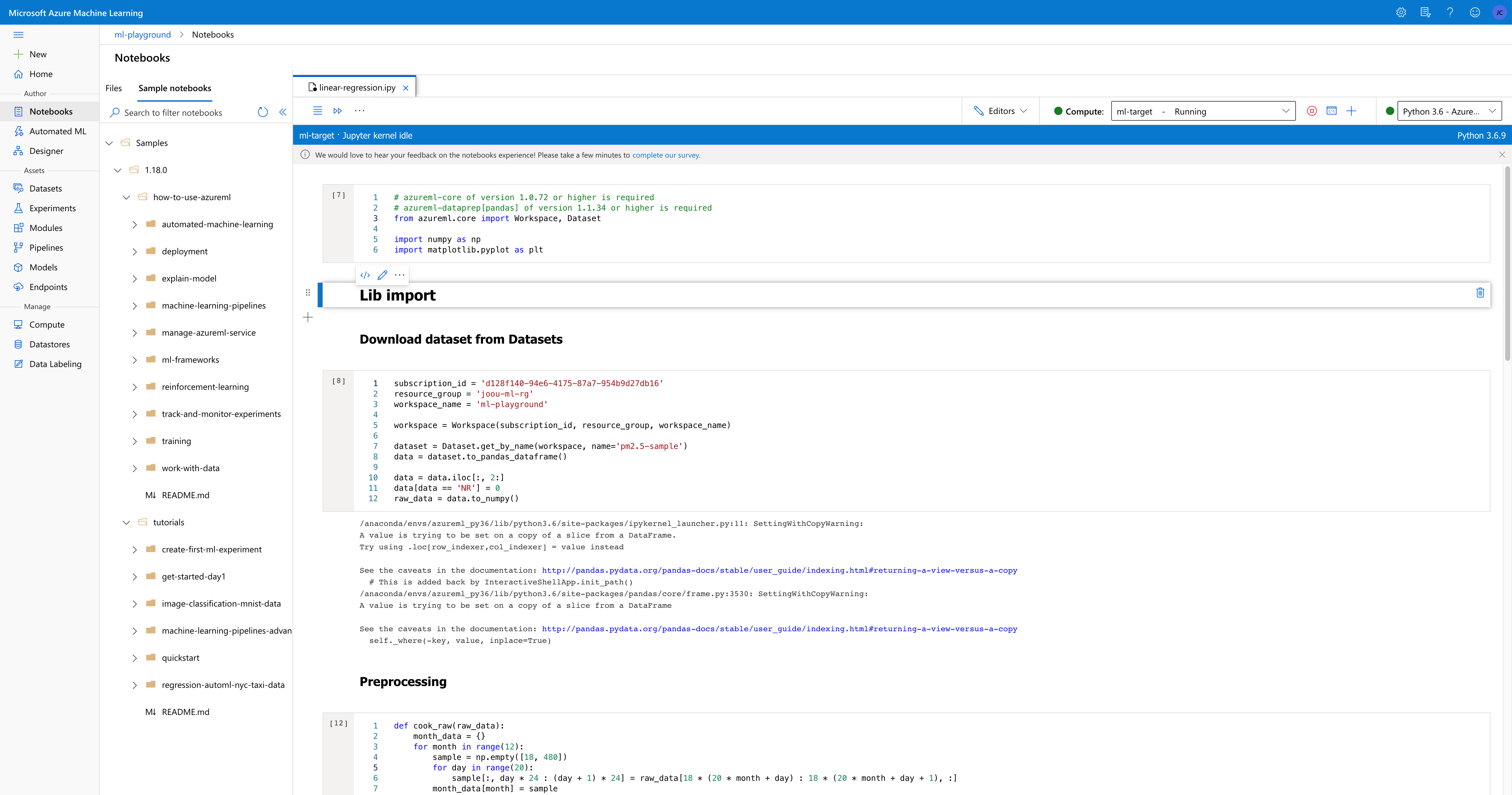
Notebooks of Azure Machine Learning Studio
Here is a brief introduction of Notebooks of AML Studio, the advantages of this product are:
- IntelliSense and Monaco Editor adopted from Visual Studio Code are great.
- Rich sample notebooks are provided, and the tab view allows user to open several documents with several file types in one page.
- An one-stop platform for user to develop their machine learning project, you can take it as cloud IDE (Integrated Development Environment). For example, user can manager their huge datasets by Datasets, and then consume them in Notebooks.
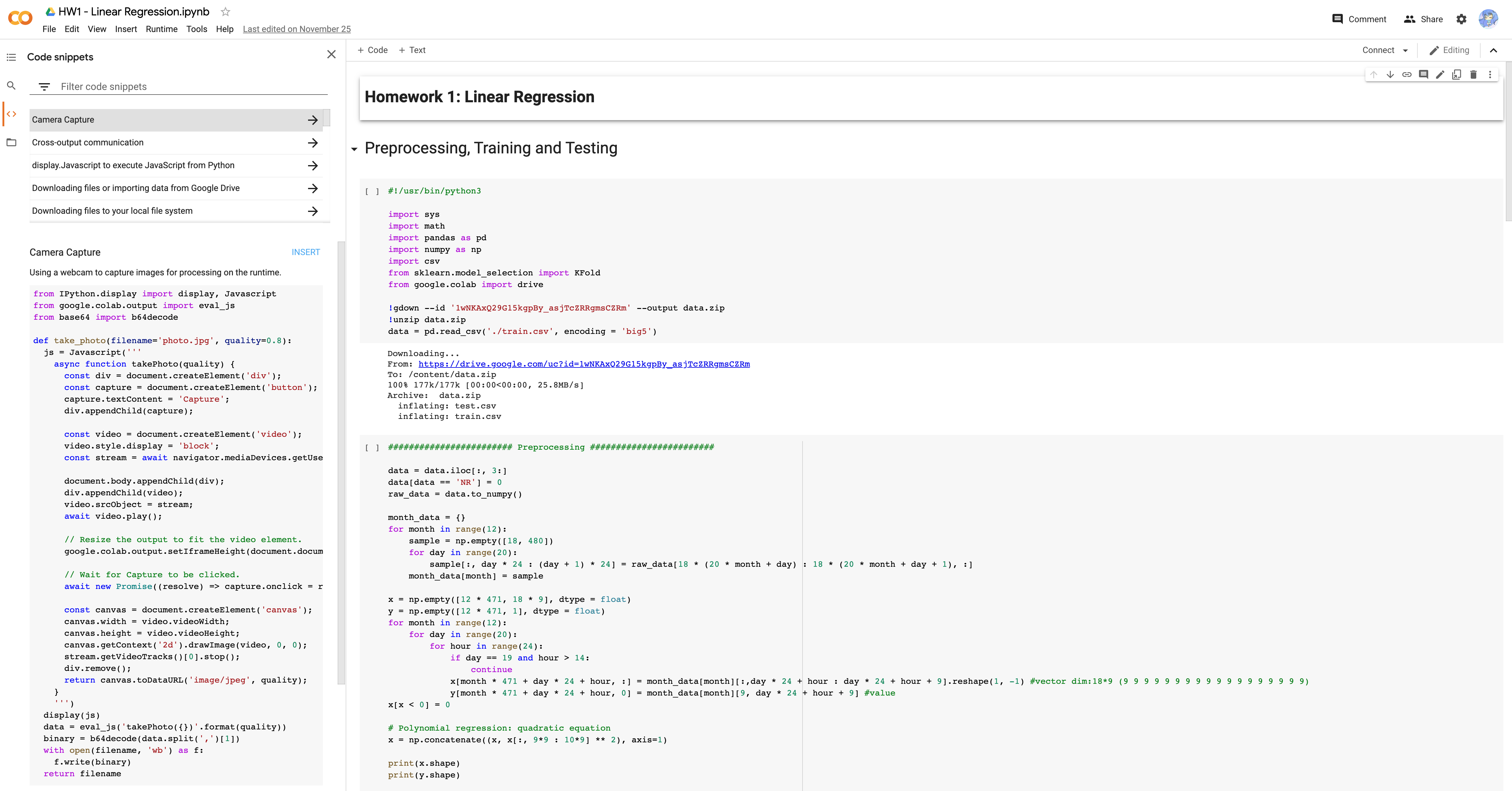
Google Colaboratory
You can open ipynb file on Google Drive by this product, there are also several advantages:
- Cleaner and larger workspace.
- “Code snippets” feature is interesting, but not smart enough (like intelligent recommendation), nor rich code exmaples.
- It will create compute target or VM (virtual machine) for the user automatically.
- Download dataset from Google Drive, comment and share are easily.
Code snippets
You can check sample code on Google Colab here, and codes below will has slight differences.
Target
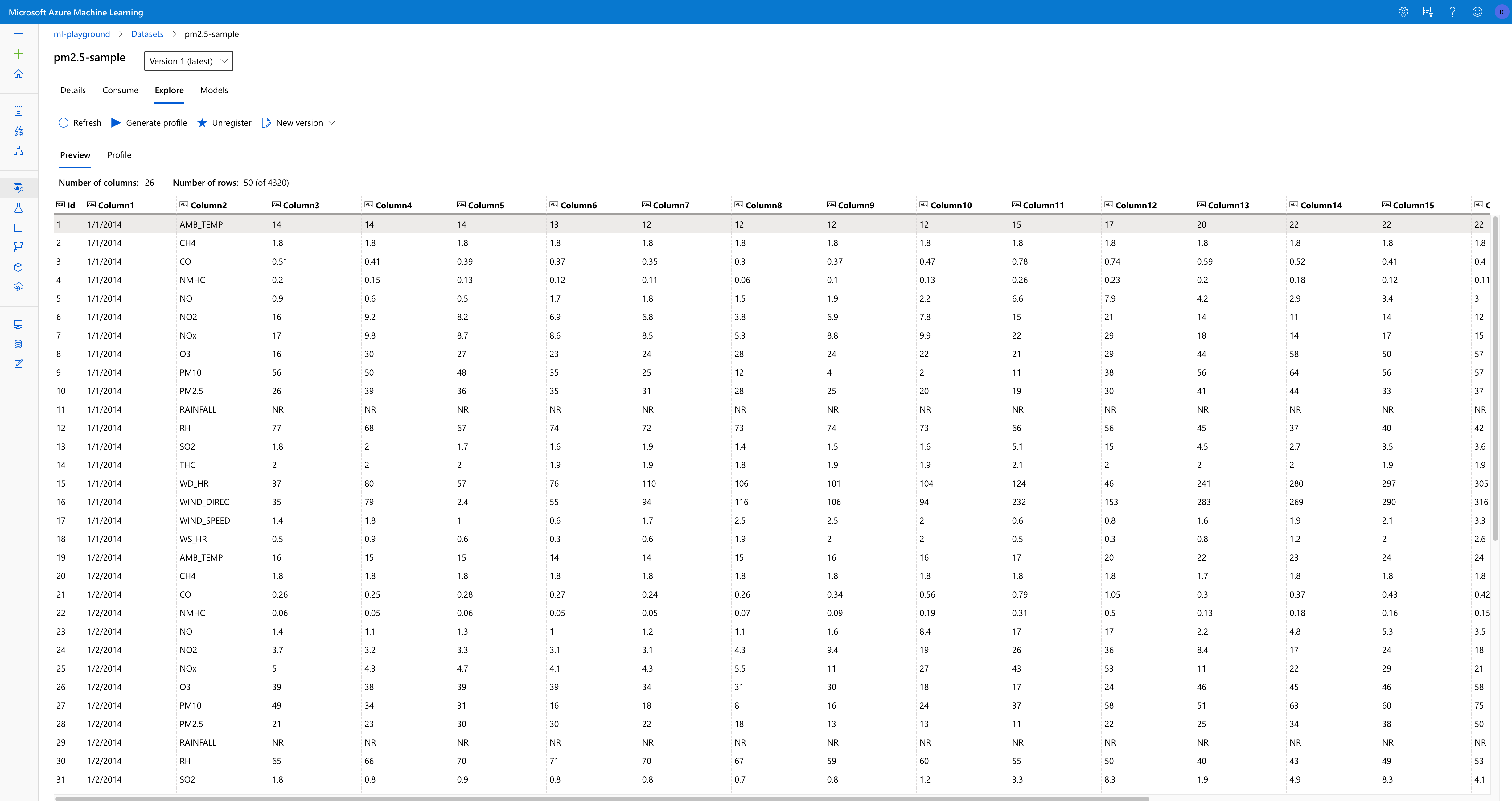
To predict the PM2.5 value of first ten hour by other nine hours data.
Data preprocessing
Original data structure looks like this:
| 00:00 | 01:00 | … | 23:00 | |
|---|---|---|---|---|
| Feature 1 of day 1 | ||||
| Feature 2 of day 1 | ||||
| … | ||||
| Feature 17 of day 1 | ||||
| Feature 18 of day 1 | ||||
| Feature 1 of day 2 | ||||
| Feature 2 of day 2 | ||||
| … |
24 columns represent 24 hours, 18 features with every first 20 days of month in one year, we have
Our target data structure of
| Feature 1 of 1st hour | Feature 1 of 2nd hour | … | Feature 1 of 9th hour | Feature 2 of 1st hour | … | Feature 18 of 9th hour | |
|---|---|---|---|---|---|---|---|
| 10th hour of day 1 | |||||||
| 11st hour of day 1 | |||||||
| … | |||||||
| 24th hour of day 1 | |||||||
| 1st hour of day 2 | |||||||
| … |
Number of columns should be
Preprocessing
You may wonder why variable
1 | # Remove first useless columns: ID, Date, Feature name |
Feature engineering by adding quadratice equation
1 | # Polynomial regression: quadratic equation |
Normalization
1 | # Normalization |
Feature engineering by pruning unimportant features
1 | # Delete features to prevent overfitting |
Split training data into training set and validation set
1 | X_train_set = X[: math.floor(len(x) * 0.8), :] |
Training and prediction
Rough training
1 | # Loss function: RMSE |
Validate training
1 | eval_loss(X_validation, y_validation, w) |
Training again and remove outliers
1 | w = train(X = X_pruned, y = y, w = w) |
Review
Compare the Steps of machine learning section with each code snippets below and rethink the whole flow, you may have an overview about machine learning now 👍 .
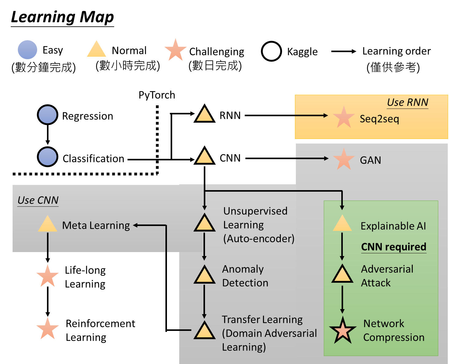
Going further
- Enjoy the References and resources
- Try assignments in the referred book and courses
![Learning map, https://bit.ly/3mf7jCU]()
References and resources
- Book: Hands-on Machine Learning with Scikit-Learn, Keras, and TensorFlow, 2nd Edition (try it free by your Microsoft account)
- Average rating 9.9 on Douban Book (till 11/24/2020)
- Errata
- Courses:
- Machine Learning 2020, Hung-yi Lee
- Machine Learning Crash Course, Google
- Desserts: Two Minute Papers